umma.dev

This post maps the maths and statistics used in machine learning and data science onto an actual workflow: loading data, cleaning it, analysing it statistically, modelling it, fine-tuning a pretrained model, and evaluating it. Each concept is introduced at the point it is used.

Loading and Describing Data - Descriptive Statistics

Every project begins with pandas. Before modelling, describe the data:

import pandas as pd

df = pd.read_csv("house_prices.csv")
df.describe()

.describe() returns mean, standard deviation, min, max and quartiles for every numeric column:

• Mean (df["price"].mean()) - the average, sensitive to outliers.
• Median (df["price"].median()) - the middle value, robust to outliers. A large gap between mean and median indicates a skewed column.
• Standard deviation (df["price"].std()) - spread of the values. Near-zero standard deviation indicates a feature carries little information and can usually be dropped.

Correlation:

df.corr(numeric_only=True)["price"].sort_values(ascending=False)

This is the correlation coefficient, applied to every column against the target. It identifies which features carry signal and flags multicollinearity (features correlated with each other, not just the target), which destabilises regression coefficients.

What “Probability” Actually Means Once There’s a Model Involved

A random variable is the outcome a model predicts: whether an email is clicked, whether a transaction is fraudulent, the next word in a sequence. A probability distribution assigns a likelihood to every possible outcome; the likelihoods sum to 1. A model does not output an answer - it outputs a distribution, and a prediction is the most likely value in it.

For example:

clf.predict_proba(X_test)
# array([[0.83, 0.17]])

This array is a probability distribution over two classes: 83% not-fraud, 17% fraud, summing to 1. For more than two classes, the softmax function generalises this:

$P(y = k) = \frac{e^{z_k}}{\sum_j e^{z_j}}$

It converts a model’s raw, unbounded output scores $z$ into a probability distribution: values between 0 and 1, summing to 1. This sits at the output layer of most classification neural networks.

Conditional probability, $P(y \mid x)$, is the probability of outcome $y$ given features $x$ - precisely what a classifier estimates. clf.predict_proba(X_test) is a numeric readout of $P(\text{fraud} \mid \text{transaction features})$.

Bayes’ Theorem

Bayes’ theorem connects a model’s confidence to the underlying reality:

$P(A \mid B) = \frac{P(B \mid A) \cdot P(A)}{P(B)}$

A medical model is 95% sensitive to a disease with 1% prevalence, and has a 5% false positive rate. Given a positive result, the probability of disease is:

prior = 0.01                    # P(disease)
sensitivity = 0.95              # P(positive | disease)
false_positive_rate = 0.05      # P(positive | no disease)

p_positive = sensitivity * prior + false_positive_rate * (1 - prior)
posterior = (sensitivity * prior) / p_positive

print(posterior)  # ~0.16

The result is approximately 16%, not 95%. Most positive results come from the large healthy population producing false positives, not from true positives in the small diseased population. A model’s confidence score cannot be interpreted without the base rate (prior) of the target: “99% accuracy” means something entirely different on a dataset with 0.1% fraud than on a balanced dataset.

GaussianNB implements Bayes’ theorem directly:

from sklearn.naive_bayes import GaussianNB

nb = GaussianNB()
nb.fit(X_train, y_train)
nb.predict_proba(X_test)

It computes $P(y \mid x)$ for each class from feature likelihoods and class priors, assuming feature independence (hence “naive”).

Cleaning and Scaling - Linear Algebra and Distributions

Missing values require an imputation strategy - a value consistent with the rest of the distribution:

df["income"] = df["income"].fillna(df["income"].median())

Median imputation is preferred over mean imputation for right-skewed columns (e.g. income), where high earners inflate the mean.

Models using gradient descent or distance metrics (e.g. k-NN) require features on comparable scales:

from sklearn.preprocessing import StandardScaler

scaler = StandardScaler()
X_scaled = scaler.fit_transform(X)

StandardScaler applies the z-score formula, $z = (x - \mu) / \sigma$, to every column, centring each feature at 0 with unit standard deviation. Without this step, a feature measured in the thousands (salary) dominates a feature measured in single digits (years of experience) by scale alone, independent of predictive value.

Data Science

Machine learning optimises for predictive performance. Classical data science asks whether a relationship in the data is real, how strong it is, and how confident an estimate can be. Both rely on the same underlying maths, applied differently.

Sanitising Raw Data

A statistic is only as trustworthy as the underlying data. Most real-world errors originate here, not in the model.

Duplicates inflate statistics derived from row counts or averages:

df = df.drop_duplicates()

Missing and invalid values:

df.isna().sum()
df["signup_date"] = pd.to_datetime(df["signup_date"], errors="coerce")

errors="coerce" converts invalid dates to NaT rather than raising an error or silently retaining bad data; these then appear in the .isna().sum() count.

Outlier detection. The IQR (interquartile range) method flags values outside the middle 50% of the data:

Q1 = df["price"].quantile(0.25)
Q3 = df["price"].quantile(0.75)
IQR = Q3 - Q1

outliers = df[(df["price"] < Q1 - 1.5 * IQR) | (df["price"] > Q3 + 1.5 * IQR)]

The z-score method flags values an unusual number of standard deviations from the mean:

z_scores = (df["price"] - df["price"].mean()) / df["price"].std()
outliers = df[z_scores.abs() > 3]

Neither method implies deletion by default - a genuine £2,000,000 house is not a data error. These methods surface candidates for review, not automated decisions.

Regression as Inference

sklearn.linear_model.LinearRegression (below) optimises for prediction: coefficients and a .predict() method. Classical statistics asks whether the relationship is real and how confident the estimate is - the purpose of statsmodels:

import statsmodels.api as sm

X_with_const = sm.add_constant(X)  # adds the intercept term
model = sm.OLS(y, X_with_const).fit()
print(model.summary())

model.summary() reports statistics sklearn does not surface:

• Coefficient and standard error - the estimated effect of each feature, and how uncertain that estimate is.
• p-value per coefficient - tests the null hypothesis that the feature has no effect on the target ($\theta_i = 0$). A small p-value indicates the relationship is unlikely to be due to chance.
• Confidence interval per coefficient - the plausible range for the true effect size, not just a single point estimate.
• R-squared - the proportion of variance in the target explained by the model:

$R^2 = 1 - \frac{\sum(y_i - \hat{y}_i)^2}{\sum(y_i - \bar{y})^2}$

An R-squared of 0.7 indicates the model explains 70% of the variation in the target; the remaining 30% is unexplained. Adjusted R-squared penalises additional predictors, since R-squared increases monotonically with added features regardless of relevance.

Residual plots (actual minus predicted values) test whether a linear model is appropriate:

residuals = y - model.predict(X_with_const)
import matplotlib.pyplot as plt
plt.scatter(model.predict(X_with_const), residuals)

A patternless scatter around zero indicates a good fit. A curve or funnel shape indicates non-linearity or non-constant error variance (heteroscedasticity), either of which invalidates the p-values and confidence intervals above, even if the coefficients appear reasonable.

Linear Regression for Prediction

The full prediction pipeline:

from sklearn.linear_model import LinearRegression
from sklearn.model_selection import train_test_split

X_train, X_test, y_train, y_test = train_test_split(X_scaled, y, test_size=0.2)

model = LinearRegression()
model.fit(X_train, y_train)

print(model.coef_)       # theta_1 ... theta_n
print(model.intercept_)  # theta_0

model.fit() minimises Mean Squared Error:

$L(\theta) = \frac{1}{m}\sum_{i=1}^{m}(\hat{y}_i - y_i)^2$

LinearRegression solves this directly via the normal equation, a closed-form matrix calculation, because the cost function has a single minimum. Models without a closed-form solution (logistic regression, neural networks) require iterative gradient descent instead - hence the max_iter parameter on those models but not on LinearRegression.

SGDRegressor exposes gradient descent explicitly:

from sklearn.linear_model import SGDRegressor

sgd = SGDRegressor(learning_rate="constant", eta0=0.01, max_iter=1000)
sgd.fit(X_train, y_train)

eta0 is the learning rate $\alpha$ in $\theta_{new} = \theta_{old} - \alpha \nabla L(\theta_{old})$. Too high, and sgd.fit() fails to converge; too low, and max_iter is exhausted before convergence.

Regression Types and When to Use Each One

Regression is a family of algorithms, not a single one. The same dataset produces different fits depending on which is used:

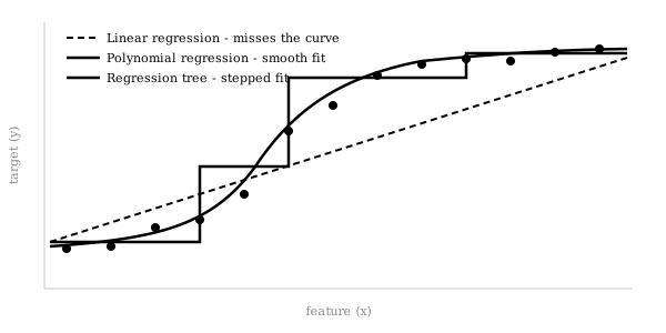
Linear regression assumes a straight-line relationship. Default first model for a continuous target; baseline for comparison.

Polynomial regression fits non-linear relationships (accelerating sales, a plateauing dose-response curve) by feeding transformed features (x, x², x³, …) into linear regression:

from sklearn.preprocessing import PolynomialFeatures
from sklearn.linear_model import LinearRegression
from sklearn.pipeline import make_pipeline

poly_model = make_pipeline(PolynomialFeatures(degree=2), LinearRegression())
poly_model.fit(X_train, y_train)

A high degree fits noise rather than signal - the overfitting problem regularisation addresses.

Ridge regression (L2 regularisation) addresses multicollinearity, which destabilises linear regression coefficients. It adds a penalty on coefficient magnitude to the cost function:

$L(\theta) = \text{MSE} + \lambda\sum_{i=1}^{n}\theta_i^2$

from sklearn.linear_model import Ridge

ridge = Ridge(alpha=1.0)
ridge.fit(X_train, y_train)

Coefficients shrink toward zero without reaching it. Appropriate when most features contribute genuine signal and stability is the priority.

Lasso regression (L1 regularisation) uses the absolute value of the coefficients instead of the square:

$L(\theta) = \text{MSE} + \lambda\sum_{i=1}^{n}|\theta_i|$

from sklearn.linear_model import Lasso

lasso = Lasso(alpha=0.1)
lasso.fit(X_train, y_train)

Unlike Ridge, Lasso can shrink coefficients exactly to zero, performing feature selection. Appropriate for high-dimensional data where only a subset of features is expected to matter.

Elastic Net combines both penalties, applying feature selection while handling correlated feature groups better than Lasso alone:

from sklearn.linear_model import ElasticNet

elastic = ElasticNet(alpha=0.1, l1_ratio=0.5)
elastic.fit(X_train, y_train)

l1_ratio controls the mix - 1.0 is pure Lasso, 0.0 is pure Ridge.

Poisson regression models count targets (website visits, insurance claims, support tickets). Linear regression can predict negative counts, which are invalid; Poisson regression is constrained to non-negative integer-valued targets:

from sklearn.linear_model import PoissonRegressor

poisson = PoissonRegressor()
poisson.fit(X_train, y_train)

Regression trees and ensembles do not fit a global equation. A decision tree regressor recursively splits the data by feature thresholds and predicts the mean target value within the resulting group - the step function in the diagram above.

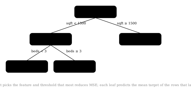
Each split minimises MSE across the resulting groups. For a node $S$ split into groups $L$ and $R$, the tree searches every feature and threshold to maximise:

$\Delta = \text{MSE}(S) - \left(\frac{|L|}{|S|}\text{MSE}(L) + \frac{|R|}{|S|}\text{MSE}(R)\right)$

This search repeats recursively within $L$ and $R$ until a stopping rule is reached. Each leaf predicts the mean target value of its training rows:

from sklearn.tree import DecisionTreeRegressor

tree = DecisionTreeRegressor(max_depth=4, min_samples_leaf=20, min_samples_split=40)
tree.fit(X_train, y_train)

These stopping-rule parameters implement the bias-variance tradeoff. max_depth limits split depth: too shallow underfits (high bias); too deep memorises the training set (high variance). min_samples_leaf and min_samples_split prevent leaves small enough to represent individual memorised rows rather than a generalisable group.

A single tree overfits despite these controls. Two ensemble methods address this, both building on maths covered above; single decision trees are rarely deployed in practice.

Random forests train many trees, each on a bootstrap resample of the rows and a random subset of features per split. Averaging decorrelated trees cancels individual overfitting - the same law of large numbers logic behind averaging cross-validation folds.

from sklearn.ensemble import RandomForestRegressor

rf = RandomForestRegressor(
    n_estimators=200,
    max_depth=6,
    max_features="sqrt",
    oob_score=True,
)
rf.fit(X_train, y_train)
print(rf.oob_score_)

max_features decorrelates the trees; without it, every tree splits on the same dominant feature first, defeating the purpose of averaging. oob_score provides free validation: each tree leaves roughly a third of the data out-of-bag, usable for validation without a separate train/test split.

Gradient boosting trains shallow trees sequentially, each fit to the residuals of the previous trees - gradient descent performed over trees rather than a weight vector.

from sklearn.ensemble import GradientBoostingRegressor

gbr = GradientBoostingRegressor(
    n_estimators=500,
    learning_rate=0.03,
    max_depth=3,
    subsample=0.8,
)
gbr.fit(X_train, y_train)

learning_rate is $\alpha$ from gradient descent, scaling each tree’s correction. Smaller values require more n_estimators but generalise better than large, aggressive corrections. subsample=0.8 trains each tree on a random 80% of rows, reducing overfitting further.

Feature importance is derived directly from tree-based models:

importances = pd.Series(rf.feature_importances_, index=X.columns).sort_values(ascending=False)

This sums the MSE reduction attributable to each feature across all splits and trees. Unlike the correlation coefficient, which only detects linear relationships, this captures non-linear and interaction effects.

Production systems typically use XGBoost, LightGBM or CatBoost: the same algorithm, engineered for speed, with built-in handling of missing values (and, in CatBoost, categorical features without one-hot encoding):

import xgboost as xgb

model = xgb.XGBRegressor(n_estimators=500, learning_rate=0.03, max_depth=4)
model.fit(X_train, y_train)

Tree-based regression is appropriate for relationships with kinks, interactions or thresholds difficult to encode via polynomial features, mixed numeric/categorical features, or when scaling is undesirable (trees split on raw thresholds, so StandardScaler is unnecessary). The cost is interpretability: a single tree is readable as a flowchart, but an ensemble of hundreds of trees is a black box; feature_importances_ is the closest available explanation.

Logistic regression, despite the name, is used for classification, not continuous prediction.

Classification - Logistic Regression and the Sigmoid

Classification uses the same workflow with a different model and loss function:

from sklearn.linear_model import LogisticRegression

clf = LogisticRegression()
clf.fit(X_train, y_train)

clf.predict_proba(X_test)  # the distribution from the probability section above

The sigmoid function converts the raw linear output into a probability:

$\sigma(z) = \frac{1}{1 + e^{-z}}$

LogisticRegression minimises log loss (cross-entropy), not MSE, which produces calibrated probabilities; a linear regression fit to 0/1 labels does not.

Evaluating a Model - Inferential Statistics

Accuracy is misleading on imbalanced data (see the disease example above, where a 95%-sensitive test was correct only 16% of the time on a positive result):

from sklearn.metrics import confusion_matrix, classification_report

print(confusion_matrix(y_test, clf.predict(X_test)))
print(classification_report(y_test, clf.predict(X_test)))

classification_report returns precision, recall and F1 score - different weightings of the confusion matrix that accuracy does not capture.

Cross-validation applies the Central Limit Theorem in practice:

from sklearn.model_selection import cross_val_score

scores = cross_val_score(clf, X_scaled, y, cv=5)
print(scores.mean(), scores.std())

A single train/test split produces one score, which may reflect chance. Five splits, evaluated by mean and standard deviation, yield an approximate confidence interval - the difference between “94% accuracy” and “94% ± 2% accuracy.”

Fine-Tuning a Hugging Face Model

Fine-tuning a pretrained Hugging Face model uses the same gradient descent loop as SGDRegressor, at larger scale with a more sophisticated optimiser:

from transformers import AutoTokenizer, AutoModelForSequenceClassification, Trainer, TrainingArguments

model_name = "distilbert-base-uncased"
tokenizer = AutoTokenizer.from_pretrained(model_name)
model = AutoModelForSequenceClassification.from_pretrained(model_name, num_labels=2)

def tokenize(batch):
    return tokenizer(batch["text"], padding=True, truncation=True)

train_dataset = dataset["train"].map(tokenize, batched=True)

args = TrainingArguments(
    output_dir="./results",
    learning_rate=2e-5,
    per_device_train_batch_size=16,
    num_train_epochs=3,
)

trainer = Trainer(model=model, args=args, train_dataset=train_dataset)
trainer.train()

Each argument corresponds to a specific mathematical component:

• learning_rate=2e-5 - $\alpha$ from gradient descent. Fine-tuning uses a smaller learning rate than training from scratch, since pretrained weights are already near a good solution; large steps degrade them.
• num_train_epochs - full passes over the training data. Each pass computes cross-entropy loss between predicted class probabilities (the softmax distribution above) and true labels, then backpropagates the error via the chain rule.
• per_device_train_batch_size - the gradient is averaged over a batch rather than the full dataset (impractical) or single examples (too noisy). The batch gradient is a noisy but usable estimate of the true gradient, by the law of large numbers.
• Trainer defaults to the Adam optimiser, which maintains a running average of past gradients (momentum) and adapts the learning rate per parameter, converging faster and more reliably than plain gradient descent.

trainer.train() logs the loss at each step: $L(\theta)$ from the linear regression section, computed on token predictions.

Estimating Uncertainty - Monte Carlo Methods in Practice

Cross-validation above uses repeated sampling for an accuracy estimate. Two further Monte Carlo techniques are common in practice:

Bootstrapping a confidence interval, without assuming any particular distribution:

import numpy as np

accuracies = []
for _ in range(1000):
    sample = df.sample(frac=1, replace=True)
    X_s, y_s = sample.drop("target", axis=1), sample["target"]
    accuracies.append(clf.score(X_s, y_s))

lower, upper = np.percentile(accuracies, [2.5, 97.5])
print(f"95% CI: [{lower:.3f}, {upper:.3f}]")

This resamples the dataset with replacement 1000 times, scoring the model each time, and takes the 2.5th and 97.5th percentiles as a 95% confidence interval, without a closed-form formula.

Monte Carlo dropout, for an uncertainty estimate from a neural network at prediction time:

import torch

model.train()  # keep dropout active, even though we're predicting
preds = torch.stack([model(x_input) for _ in range(50)])
mean_pred = preds.mean(0)
uncertainty = preds.std(0)

Running the same input through the model 50 times with dropout active produces 50 distinct predictions. The mean is the point estimate; the standard deviation is an estimate of predictive uncertainty, useful for flagging low-confidence predictions.

Maths Topics

A reference mapping each topic to where it applies:

• Descriptive stats (mean, median, std dev, correlation) - every df.describe() and df.corr() call, at the start of any project.
• Probability distributions, conditional probability, Bayes’ theorem - what predict_proba returns, why confidence scores diverge from real-world accuracy, and how GaussianNB operates.
• Vectors, matrices, dot products - how a row of data and a dataset are represented and fed into any model, from linear regression to a transformer.
• Norms and scaling (z-scores) - StandardScaler, and any model using gradient descent or distance calculations.
• IQR and z-score outlier detection - data sanitation, before any statistic derived from the data can be trusted.
• Derivatives, gradients, the chain rule - .fit() on anything beyond plain linear regression, and backpropagation during fine-tuning.
• Cost/loss functions (MSE, cross-entropy) - the number Trainer logs at each step, and the target of learning_rate and num_train_epochs.
• Regularisation (L1/L2 penalties) - Ridge, Lasso and ElasticNet, and which to use when features are correlated or feature selection is needed.
• Recursive splitting and bootstrap aggregation - DecisionTreeRegressor, RandomForestRegressor and GradientBoostingRegressor, for relationships a straight line or polynomial cannot capture.
• R-squared, p-values, confidence intervals on coefficients - statsmodels.OLS.summary(), and the distinction between predictive accuracy and statistical significance.
• Central Limit Theorem and confidence intervals on metrics - cross_val_score, and reading model results as a range rather than a single number.
• Hypothesis testing and p-values - A/B testing a model change or product feature before deployment.
• Monte Carlo sampling and bootstrapping - estimating uncertainty around a metric without a closed-form formula.